Algorithms Used for Data Processing in FTIR
In this article, I will present some of the algorithms used for a variety of data processing operations applied to spectra in FTIR. These algorithms are adopted in IRsolution software.
Smoothing
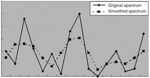
Fig. 1 Simple Smoothing Based on Replacement with Average Values
Smoothing is a process used to smoothen the shape of spectra.
For example, applying this process to a spectrum with a low S/N ratio makes it possible to reduce the influence of noise.
Although the peak resolution decreases, the existence of peaks becomes easier to ascertain and the overall shape of the spectrum becomes clearer. So, in the analysis of unknown samples, this process is effective for obtaining qualitative information.
Smoothing a spectrum involves reducing the degree with which the spectral intensity changes at individual data points. A very simple way of smoothing would be to replace the intensity value of each individual data point with the value obtained by averaging the intensities of three points, which consist of the data point itself and two neighboring points. This does, to a degree, achieve the desired effect. In the figure shown below, the dotted line graph represents the result of applying this process to the solid line graph. The degree with which the spectrum changes at each point is reduced.
IRsolution uses a slightly more complex algorithm. Instead of taking the average of three points, it uses the value obtained by multiplying the intensity of each one of a specified number of smoothing points by a weighting factor and totaling the values thus obtained. This process is referred to as the application of a "third-order Savitzky-Golay smoothing filter" and the factors are determined by a function that is
largest at the original data point and decreases as one moves away from this point. The number of smoothing points can be specified in IRsolution's smoothing command window. If this is set to a large value, the weighted average for data points covering a wide range is obtained and, in general, a smoother spectrum, with relatively few bumps, is produced.
Interpolation
Interpolation is a process for obtaining spectral intensities at locations with no original data points from the spectral intensities of surrounding data points. It increases the number of data points.
This process is used, for example, when comparing two sets of data that have data points at different intervals because the original data was obtained with different resolutions. By applying the appropriate form of interpolation, the sizes of the intervals between data points can be unified.
There is a simple type of interpolation algorithm in which two points are joined by a straight line and a new point is created on that line. IRsolution, however, uses an algorithm based on the Laplace-Everett formula. This is an interpolation algorithm that creates new points using the intensities of several surrounding points, not just the neighboring points, and thereby reflects the trends of curves over a relatively wide range. With IRsolution, four surrounding points are used.
As an example, suppose that there are four points, P0, P1, P2, and P3 (in order), on a spectral curve and that their intensities are, respectively, I0, I1, I2, and I3. If P is a point that divides P1 and P2 internally in the ratio t:1-t, the intensity at P obtained with simple interpolation is as follows:
However, the intensity obtained with the IRsolution algorithm is as follows:
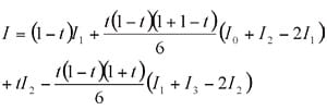
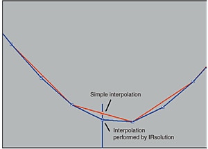
Fig. 2 Interpolation Based on Laplace-Everett Formula
IRsolution's interpolation function not only allows the sizes of the data intervals to be decreased by a specified factor (e.g., to intervals of one half or one quarter the size), but also makes it possible to switch to data intervals of any specified size. This is possible because the function obtains a curve using the original data points, and creates new data points by obtaining the intensities at the new specified data intervals. For this reason, even if the original data interval is a multiple of the new specified data interval, and data wavenumbers of the old and new data happen to coincide, the respective intensities will, in general, be slightly different.
It must be remembered that interpolation is only a mathematical method for estimating intensity values and the values obtained may differ from the actual intensities.
Peak Detection
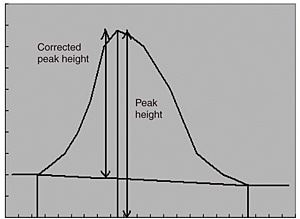
Fig. 3 Peak Height and Corrected Peak Height
Peak detection involves the identification of absorbance at specific wavenumbers in a spectrum, and is used for the qualitative and quantitative analysis of sample substances.
With IRsolution, the threshold value, the noise level, and the minimum area are required as parameters for peak detection. (Although these values differ according to whether the vertical axis of the spectrum represents transmittance or absorbance, the basic principle is the same. Here, an example where the vertical axis represents absorbance is used.)
First, the first- and second-order derivatives of the spectrum are calculated and the result is saved. Next, using these results, the wavenumber positions on the spectrum at which the first-order derivative changes from a positive to a negative value are detected, and these are considered to be peak candidates (because it is possible that they are positions where the spectrum takes maximum values).
From these peak candidates, the ones for which the absorbance does not attain the threshold value are
discarded. Then, the difference in first-derivative value between each candidate point and points before and after it is calculated, and the points for which the absolute value of this difference does not attain the specified noise level are judged to be noise and are discarded.
Among points before and after the remaining peak candidates, points for which the first-order derivative changes from a negative value to a positive value and for which the second-order derivative is negative are searched for. If such points are found, they are judged to be the "valleys" before and after peaks. If valleys are not found, the corresponding candidates are judged to not be peaks and discarded. The valleys found before and after the peak candidate points are joined to form baselines, and the heights and areas of the corrected peaks are calculated. If these two values are greater than the specified threshold and minimum area respectively, the corresponding points are judged to be peaks.
The operations are basically the same in the case where the vertical axis represents transmittance. The transmittance values at the peak bottoms (rather than the peak tops), the depths of these peak bottoms from the baseline, and the areas bound by peaks and the 100% line and by peaks and the baseline are used instead.
Film-Thickness Calculation
This function calculates, from the number of interference fringes in a specified wavenumber range, the thickness of a film through which infrared light passes. In terms of algorithms, this function can be thought of as simple peak detection and its application.
As with standard peak detection, the first-order derivative of the spectrum is calculated, and the places where its value changes from positive to negative are detected. Precise noise level checks are not performed on the spectrum. Such characteristics are regarded as peaks.
The maximum and minimum peak wavenumbers in the specified wavenumber range are detected, and the number of peaks between them is counted. A calculation based on the following formula is performed on the number of counted peaks and the set refractive index and angle of incidence.
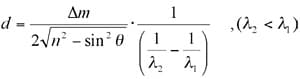
Here, "d" represents the film thickness, "λ1" and "λ2" represent the wavelengths of the peaks or valleys at either end of the specified wavenumber range, "n" represents the refractive index of the film, "θ" represents the angle of incidence of infrared light with respect to the sample, and "Δm" represents the number of peaks between "λ1" and "λ2".
Atmospheric Correction
This is a corrective function that subtracts the component of a spectrum that corresponds to absorbance due to water vapor and carbon dioxide in the atmosphere, and thereby suppresses the influence of these factors. With IRsolution, the approximate shape of the background spectrum that is displayed in power spectrum format is calculated, and using this and the absorption peaks in the original background spectrum, the water vapor and carbon dioxide peaks are canceled out.
First, the approximate shape of the background spectrum is calculated. In order to do this, figures entered for water vapor and carbon dioxide in both the high and low wavenumber ranges via the parameter setting window are used. These figures are scale factors expressed as wavenumbers that are used to perform coarse graining of the spectrum. In the respective wavenumber regions, changes in small wavenumber ranges not exceeding the set figures are ignored, and an outline spectrum with no fine absorption peaks is calculated.
The wavenumber ranges are as follows:
High wavenumber range for water vapor:
3,540 to 3,960 cm-1
Low wavenumber range for water vapor:
1,300 to 2,000 cm-1
High wavenumber range for carbon dioxide:
2,250 to 2,400 cm-1
Low wavenumber range for carbon dioxide:
600 to 740 cm-1
The resulting spectrum has the form of an envelope curve created by removing small bumps from the original background spectrum. From the difference between these spectra, an absorption peak pattern for the water vapor and carbon dioxide in the atmosphere is calculated.
Furthermore, regarding the sample spectra displayed in power spectra format, the same kind of peak pattern is calculated, and the ratio of the background spectrum to this peak pattern is obtained. Subtracting the peak pattern obtained by performing scaling with this factor from the power spectrum makes it possible to obtain a spectrum from which the influence of the water vapor and carbon dioxide in the atmosphere is eliminated. (The final spectrum is given as a ratio of the sample and background spectra.)
IRsolution's atmospheric correction function, then, performs correction using power spectra for both the background and the sample. For this reason, correction is only possible for spectra obtained with IRsolution that are in a format bearing the .smf extension.
Library Searches
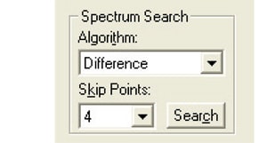
Fig. 4 Selection of Search Algorithm
Many of the algorithms used for library searches are extremely complex. It would be impossible to give an exhaustive explanation of them all in such a limited space so, here, I will describe a relatively simple type of algorithm in the context of the operation of a typical library search.
Shimadzu IRsolution software's search function supports many different types of search techniques. The most basic is called "spectrum search". When using spectrum search, various settings must be made, including the selection of the algorithm.
Various algorithms can be selected in IRsolution's spectrum search. Of these, the algorithm "Difference" is relatively simple and I will describe the operation performed when this algorithm is used.
When a spectrum search is executed with IRsolution, processing of the wavenumber range is performed first. This is a selection function whereby the sample spectrum is compared with the library spectra within a specified wavenumber range, rather than the range of the entire spectrum. This function makes it possible to perform searches using only characteristic parts of spectra. Actually, this function converts the wavenumber range expressed in cm-1 units to an index (number) of the data points that configure the spectrum, and only the data points of the applicable index are transferred to the comparison function part of the software.
Next, the spectrum is normalized in terms of intensity. This process corresponds to the "Normalize" command that is displayed on IRsolution's "Manipulation" menu. A constant factor is applied to the entire spectrum so that the maximum absorbance becomes 1 while the shape of the spectrum is preserved.
In general, the sizes of spectra of unknown samples differ from those of library spectra; therefore, this processing is necessary to facilitate comparison based on appropriate spectral forms.
After the size of the spectrum has been normalized for all the data points in the set wavenumber range, the differences in intensity between the spectrum of the unknown sample and the library spectra are obtained as absolute values, and these values are totaled. If the spectrum of the unknown sample and a library spectrum are a perfect match, this value will naturally be zero. In practice, the value varies according to the degree of similarity between the two spectra. Multiplying this value by a certain factor and subtracting it from 1,000 gives an index (the "hit quality") that will equal 1,000 in the case of a perfect match. This operation is performed on all the library spectra used, and the results are displayed as a list with the spectra arranged in decreasing order of hit quality.
The operation of other types of algorithms is basically the same. The only difference may be, for example, that instead of the absolute values of the differences between the spectrum of the unknown sample and the library spectra, the squares of the differences are used.
Summary
Here, I have given a simple explanation of the algorithms used in some of the data processing operations performed by IRsolution. In the use of data processing functions, I do not think that it is usually necessary to be aware of the precise details of operation. Understanding the algorithms, however, can help the user appreciate the effects of the corresponding processes. Sometimes, when using a data processing operation, try to be aware of the utility of the operation.