Measurement Principle / Measurement Mode
SPM Basic Knowledge Q&A
Q1-1: Could you provide an overview of SPMs?
Q1-2: What is the basic operating principle behind SPMs?
Q1-3: What are the differences between contact and dynamic modes?
Q1-4: What about various other SPM modes besides AFM modes?
Q1-5: What can be determined from the SPM phase mode?
Q1-6: What is the resolution capability of SPMs?
Q1-7: Can you explain the force curve?
Q1-1: Could you provide an overview of SPMs?
|
A: |
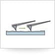
A scanning probe microscope (SPM) is a new type of microscope with a tiny needle that traces the contour of samples in order to investigate their shape or other properties. |
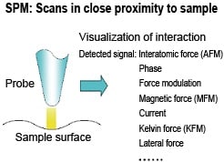
SPM is a generic term for all microscopes used to observe sample surfaces three-dimensionally by moving a tiny needle (probe), with a tip radius of only a few dozen nanometers, close to the sample surface. This is done to detect the mechanical and electromagnetic interactions between the probe and sample as it scans the sample surface (see the figure below). These microscopes are sometimes referred to by various names, such as scanning probe microscopes, probe microscopes, or SPMs. One of the most basic types of scanning probe microscope is the atomic force microscope (AFM). Another type of SPM is the scanning tunneling microscope (STM), which functions by detecting the tunneling current that flows between the probe and sample. (A tunneling current exists even without contact, due to the tunneling effect, which acts at extremely close distances.)
STM is capable of even atomic resolution, particularly in ultra-high vacuum environments, but they also have various limitations. For example, STMs are not able to observe nonconductive samples, and in atmospheric conditions, they are extremely sensitive to sample surface contamination. In contrast, atomic force microscopes detect the forces acting between the sample and probe (which are sometimes attractive and sometimes repulsive, but difficult to accurately understand). Therefore, AFMs can be used to observe samples of insulation materials. They can also observe samples easily even in atmospheric air. Consequently, AFMs are widely used, and most commercially marketed SPM systems are based on AFM principles. AFM systems can be generally categorized as using contact mode or dynamic mode. Furthermore, by simultaneously detecting other interactions between the sample and probe, some systems are now able to not only visualize the three-dimensional contours of samples, but also map various other properties. All of these types of systems are referred to as SPMs. In light of the many possible types of SPM systems, an acronym of the form "SXM" is often used, where the "X" indicates the physical quantity detected.
Invented in the 1980s, SPMs are relatively new in history. The STM was invented in 1981 and the AFM in 1986. The invention of the STM enabled clear observation of an actual spatial image of the structure of 7 x 7 Si(111) in an ultra-high vacuum. For their achievement, the inventors, Gerd Binnig and Heinrich Rohrer (at the IBM Zurich Research Laboratory), were awarded the Nobel Prize and became instantly famous, something still fresh in our minds. The SPM is different from a typical microscope, which uses beams and lenses to increase or reduce magnification, such as optical or electron microscopes. However, given certain conditions and samples, it is able to distinguish between atoms and molecules, and its magnification capacity rivals transmission electron microscopes. Another big advantage is that it can observe samples in air or liquids. Therefore, as a microscope essential for nanotechnology research, applications for SPM systems are expected to expand even further in future.
Q1-2: What is the basic operating principle behind SPMs?
|
A: |
SPMs observe sample shape or surface properties by detecting the bending and vibration characteristics of a cantilever arm, which has a tiny probe attached. |
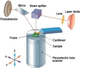
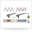
Basic Configuration of the Scanning Probe Microscope
There are many derivatives of the SPM, such as the magnetic force microscope (MFM), surface potential microscope (or Kelvin probe force microscope, KFM), or lateral force microscope (LFM), but their most fundamental principles are illustrated by the atomic force microscope (AFM).
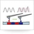
The AFM uses a cantilever (a beam anchored at only one end) with a needle-shaped tip to detect force. The tiny forces acting between the needle on the tip of the cantilever and the sample (atomic forces) cause the cantilever to vary in how it bends and vibrates. These variations are detected with high sensitivity using laser light reflected off the back side of the cantilever. At the same time, either the cantilever or sample is precisely scanned and controlled three-dimensionally by a scanner with a piezoelectric element. In general, the distance from the sample (Z-height) is fed-back and controlled so that either the amount of bending is kept constant (contact mode), or the amount of vibration is kept constant (dynamic mode), as the cantilever is scanning the sample surface (XY-plane).
A 3D contour image of the sample surface (an image used to observe the shape of the sample surface) is obtained by loading the Z-axis feedback value (output voltage to the scanner) for each scanned position (X and Y coordinates) into a computer that reconstructs the data as a 3D image. The contour image can be further processed (using offline software) to analyze any cross section of interest, by shading or false color-coding, or displaying the section in bird’s eye view mode for example, or to analyze the surface roughness. The basic system configuration is shown above.
In addition to basic AFM contour images, Shimadzu SPM models also makes it possible to use various SPM techniques to obtain images based on information from signals indicating the physical properties of sample surfaces, such as electrical current, electrical potential, hardness, or viscoelasticity. (Some of these features are optional.)
Q1-3: What are the differences between contact and dynamic modes?
|
A: |
In contact mode, the system detects the degree of cantilever bending, whereas in dynamic mode, it vibrates the cantilever. |
There are several types of AFM operating mode, but in general, these modes can be categorized as either contact mode (DC mode and static mode) or dynamic mode (resonance mode, AC mode, and dynamic modes).
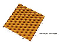
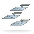
Atomic Image of Mica (Using disk-shaped air-spring isolator)
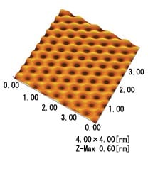
In contact mode, static atomic forces are detected based on the degree of cantilever bending, as indicated in the basic operating principles described in Q1-2. When the cantilever is moved close to the sample surface, the cantilever bends slightly due to tiny repulsive forces. Feedback control is used to stabilize the repulsive force, or in other words, to keep the degree of cantilever bending constant. The feedback values are then input to a computer to render a visual image of the surface contour. Because the repulsive forces are kept constant, this mode is also referred to as constant force mode. Due to the simple operating principle and ease of use, this has conventionally been the most common AFM mode. Due to the high resolution, this mode was also generally used for atomic and molecular-level observations of substances such as the mica sample shown below.
When observing samples using contact mode in atmospheric air, the probe scans the surface layer of the sample that has adsorbed water (contamination layer). Therefore, in addition to the repulsive forces from the sample, the cantilever can sometimes also be affected by adhesion forces (meniscus forces), which can cause noise that resemble lateral drag marks in images. Consequently, this mode is not suited to visualizing samples that tend to move, or soft surfaces.
In dynamic mode, a vertical excitation force is applied to the cantilever so that it vibrates at close to its resonant frequency. When the vibrating cantilever tip is moved close to the sample, the vibration amplitude varies. Feedback control is then used to keep the vibration amplitude constant. Since there is little chance of the probe catching on the sample during scanning, this mode is well suited to samples that tend to move, or adsorptive samples. In addition, dynamic mode cantilevers are stiffer, with a higher spring constant than contact mode cantilevers, in order to reduce the effects of static electricity. Another feature is the use of phase mode to obtain a phase signal while observing the surface contour. In recent years, dynamic mode has become a standard AFM technique.
The following is a comparison of both modes.
Comparison of Contact mode and Dynamic Mode
| Contact mode | Dynamic mode | |
|---|---|---|
| Most suitable samples | Relatively hard samples. Many restrictions. |
Comparatively soft samples with large surface irregularity. Few restrictions. |
| Cantilevers | SiN cantilevers common. Probe tip angle: Approx. 40° Comparative long service life. |
Si cantilevers common. Probe tip angle: Approx. 25° Short life under some conditions of use. |
| Resolution | Offers max. resolution for some samples and conditions. | Comparable to contact mode for a scanning range of several µm or more. |
| Related operation modes | Lateral Force (LFM), Current, Force Modulation, Force Curve | Phase, Magnetic Force (MFM), Kelvin Force (KFM) |
Q1-4: What about various other SPM modes besides AFM modes?
|
A: |
SPM modes include mechanical modes, typified by phase mode, and electrical modes, such as the electrical current mode. These make it possible to obtain images of signals based on information about the physical properties of sample surfaces. |
Recent commercially marketed SPM systems are able to obtain both sample contour images, using basic AFM mode functionality (contact and dynamic modes), and signal images, based on the physical properties of sample surfaces, such as electrical current or potential, hardness, or viscoelasticity.
Contact Mode AFM
Dynamic Mode AFM
1. Phase Mode
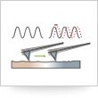
In dynamic mode, the system detects how far the phase of the detected sinusoidal cantilever vibration signal lags behind the signal of the original vibration source. These signals can then be used to create a visual image of differences in sample surface properties. The phase lag in cantilever vibration in response to sample surface properties is similar to feet sticking when walking in mud. Therefore, determining surface properties is like determining the properties of the ground based on the degree to which the feet are sticking
2. Force Modulation Mode (Viscoelasticity)
In this mode, the system vibrates the sample vertically at a constant frequency while scanning in contact mode; presses the probe against the sample; and then detects the response in terms of cantilever amplitude and phase lag. These signals can then be used to visualize differences in the viscosity and elastic properties of the sample surface.
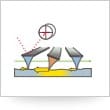
3. Current Mode
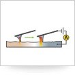
In this mode, the system applies a bias voltage between the probe and sample while scanning in contact mode, and detects the current flow between the probe and sample. It then simultaneously displays an image of the in-plane distribution of the current flow detected, along with the surface contour. This provides an image based on the localized resistance levels of the sample.
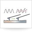
4. Magnetic Force Mode (MFM)
In this mode, the sample is scanned with a magnetized probe tip, which is vibrating near the resonant frequency, and is kept at a constant distance from the sample. This causes the cantilever amplitude and phase to vary due to repulsive and attractive forces on the probe, due to magnetic leakage from the sample surface. By detecting the amount of variation, magnetic information about the sample surface can then be visualized. This observation method is referred to as magnetic force microscopy (MFM).
5. Surface Potential Mode (KFM)
In this mode, the system measures the electric potential of the sample surface by applying an alternating current to a conductive cantilever, and then detecting the static electric force acting between the sample surface and the cantilever. This observation method is generally referred to as Kelvin probe force microscopy (KFM), or electric force microscopy (EFM).
6. Lateral Force Mode (LFM)
The sample is scanned in a direction perpendicular to the cantilever axis in contact mode, and the torsion on the cantilever is detected in order to visualize the lateral forces (friction) acting between the probe and sample. This observation method is generally referred to as lateral force microscopy (LFM), or friction force microscopy (FFM).
7. Force Curve
In this mode, the system measures and graphs the force acting on the probe (how far the cantilever bends) as the distance between the probe and sample is varied, which is referred to as force curve measurement. This mode is used to measure the adsorption and relaxation forces on the sample. It is also used for detailed cantilever selection, and to verify properties.
8. Vector Scan
In this mode, the probe is used to mark sample surfaces with letters or graphics. Examples include mechanical methods that carve the surface, and electric methods that anodize the surface. This process is also referred to as nanolithography.
Q1-5: What can be determined from the SPM phase mode?
|
A: |
Phase mode enables the visualization of differences in sample surface properties, and is particularly useful for observing the distribution of viscoelasticity in polymer materials. |
Phase mode, which is commonly used at the same time as AFM dynamic mode, can be used to obtain four signals: namely the cantilever amplitude (A), the phase lag between the applied and detected cantilever vibration signal (δ), A sine δ, and A cos δ. An image of differences in sample surface properties can then be visualized based on these signals. This is particularly useful for observing the viscoelasticity of polymers. An example is illustrated below. The phase image (right) clearly shows differences in material properties by phase, while the surface contour image (left) does not.
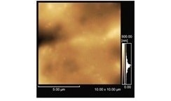
Surface Contour Image
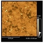
Phase Image
Contour and Phase Images of a Polymer Blend (Copolymer)
This example shows a sharp image of the blended structure of rubber. Phase mode is evidently an extremely useful detection method.
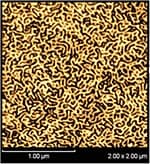
Blended Structure of Rubber
The amplitude (A) and phase (δ) are calculated from the A sine δ and A cos δ signals. In general, elastic components are dominant in A cos δ images, whereas viscous components are dominant in A sine δ images. However, this is not always the case. The phase (δ) is equivalent to the viscoelasticity image (mixed viscosity and elasticity image) and the amplitude is equivalent to the deviation image. In addition, surface contour effects can overlap with phase, A sine δ, and A cos δ.
Phase (δ) can also be expressed in terms of angular degrees. However, such values are not absolute values, but rather indicate relative variations within the same image. Therefore, such image data is qualitative, and cannot be directly compared to values in different images in general.
Signal Types Obtained in Phase Mode
| Signal | Amplitude (A) | Phase ( δ ) | A sin δ | A cos δ |
|---|---|---|---|---|
| Description of Signal | Deviation Image | Viscoelasticity (mixed image of viscosity and elasticity), surface contour, etc. | Emphasized viscous components,s urface contour,etc. | Emphasized elastic components, surface contour , etc. |
Q1-6: What is the resolution capability of SPMs?
|
A: |
There are multiple definitions for SPM resolution (theoretical resolution, control resolution, and image resolution). Many SPMs indicate a nominal resolution of 0.2 nm horizontally and 0.01 nm vertically, but this is a theoretical resolution. |
Resolution for SPMs is defined differently from spatial resolution defined for other microscopes (such as the ability to resolve between two points). This is because a reference sample (or ruler) small enough to measure lengths equivalent to the size of atoms and molecules or smaller, such as 0.01 nm or 0.2 nm, still does not exist. Academically, the expression “atomic resolution” is preferred. When discussing the spatial resolution of SPM systems, it is still necessary to think of theoretical resolution, control resolution, and image resolution separately. Many SPMs claim a nominal resolution of 0.2 nm horizontally and 0.01 nm vertically, but this is a theoretical resolution.
(1) Theoretical Resolution*
Theoretical resolution is calculated as follows. First, assume It = ∝exp (-Z/L), where It equals the detected physical quantity, Z equals the distance from probe tip to sample surface, and L equals the decay distance. Based on this assumption and given an in-plane resolution δx, height resolution δz, and a signal-to-background ratio n, then δz = L/n and δx = √{δz(2Z+ΔZ)}.
Given typical values of Z = 1 nm, L (decay distance) = 0.05 nm, and n = 5, and assuming a sufficiently small radius of curvature for the probe tip, then theoretical resolution values of δx = 0.2 nm and δz = 0.01 nm are obtained.
* Source: Noncontact Atomic Force Microscopy, written and edited by Seizo Morita, published by Maruzen.
(2) Control Resolution
Control resolution indicates the minimum step width per bit for digitally controlled systems. Control resolution depends on the scan range of the scanner, and the digital control precision (number of bits). For example, using the Shimadzu SPM-9600, the control voltage resolution in the Z-direction (height direction) is 26 bits, and the control voltage resolution in the XY-plane is 16 bits. Given the standard scanner (XY: 30 µm square max. and Z: 5 µm max.), resolution in the XY-plane is 0.076 nm and resolution in the Z-direction is 0.00006 nm, which indicates that control performance clearly exceeds the theoretical resolution. However, beware that many overseas manufacturers report the control resolution as the instrument resolution. To improve the actual resolution, the performance of the analog system must also be considered, and it is essential that the noise level of the measuring system be sufficiently low to ensure adequate atomic resolution.
(3) Image Resolution
In reality, what is referred to as atomic resolution for SPM systems is often based on data obtained from the cleavage face of lamellar crystals (such as mica and HOPG) using contact mode. Cleaving samples into layers results in atomically-smooth clean surfaces, which makes it much easier to obtain an image of lattice periodicity at the atomic scale. A so-called atomic image of the cleavage face of mica is shown below. It is referred to as an atomic image because the lattice size (5.2 Å) is consistent with the lattice constant obtained using X-ray diffraction or other methods. This image can be interpreted as a periodic signal generated from a kind of moire striping or stick-slip phenomenon, resulting from the arrangement of atoms in the clean sample face, and the arrangement of atoms in the probe tip. Note that this does not mean that the probe tip is able to enter the indentations of the periodicity; rather, it simply means that it recognizes the periodicity of the arrangement. Research aimed at achieving true atomic resolution has been continuing in recent years, with efforts that are pushing the limits of sensitivity using frequency modulation AFM (FM-AFM).
Q1-7: Can you explain the force curve?
|
A: |
During force curve measurement, the force acting on the cantilever is measured while sweeping the cantilever in the vertical (Z) direction close to the sample and changing the distance between the sample and the cantilever. The distance vs. force graph obtained by the force curve measurement is simply referred to as the force curve. |
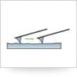
(1) Cantilever Sweeping Process
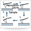
With the horizontal (XY) scan stopped at a fixed point above the sample, the cantilever is moved close to the sample (approach), and then moved away (release). This process is performed repeatedly. The forces acting on the cantilever in this sweep process are shown schematically in Fig. 1.
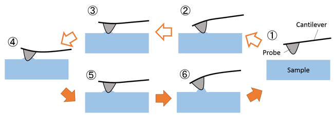
Fig. 1 Forces Acting on the Cantilever During Force Curve Measurement
| • The cantilever approaches the sample. | ||
| 1) | The probe on the cantilever tip and the sample are completely separated. | |
| 2) | The cantilever is subjected to a slight attractive force from the sample and bends downward. This is referred to as jump-in. (In some cases, there is no attractive force.) | |
| 3) | As the approach continues, the cantilever is subjected to a repulsive force and bends upward. | |
| 4) | At this point, the contact between the cantilever and the sample is the strongest, and the repulsive force is at a maximum. | |
| • The cantilever is released from the sample. | ||
| 5) | The force acting on the cantilever changes from repulsion to attraction. | |
| 6) | At this point, an adhesive force acts between the cantilever and the sample, and the attractive force is at a maximum. (In some cases, there is no adhesive force.) Immediately after this, the probe separates from the sample. This is referred to as jump-out. |
|
| 1) | The probe and the sample are completely separated again. | |
(2) How to View the Force Curve
Fig. 2 shows a typical force curve. The horizontal axis represents the Z position [Z]. The further to the right, the greater the distance between the cantilever and the sample, and the further to the left, the smaller the distance between them. The vertical axis represents the force [F] acting on the cantilever. The force is repulsive when it is above 0, and attractive when it is below 0. Points 1) to 6) in Fig. 2 correspond to those in Fig. 1, and the force acting on the cantilever at each of the points 1) to 6) in Fig. 1 can be read from Fig. 2.
By measuring the force curve, the following can be determined.
| • Adhesive force: | Force acting immediately prior to jump-out | |
| • Sample hardness: | The greater the slope (△F/△Z) at point 3) or 5), the greater the hardness of the sample. |
If the optional Nano 3D Mapping system is used, a greater variety of measurements and analyses can be performed.

Fig. 2 Typical Force Curve
During actual force curve measurements using a Shimadzu SPM series instrument, the vertical axis of the window displays a voltage [V] as shown in Fig. 3. The value on the vertical axis can be converted into force using the slope of the force curve and the spring constant of the cantilever.
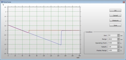
Fig. 3 Example of Force Curve Measurement Window